Plant Disease Classification using AlexNet

Introduction

Agriculture is the main source of food in India. During the crop cycle, many plant diseases can occur and can affect the crop. Identification and classification of plant disease at the leaf level is a crucial part. Traditionally, the classification of plant diseases has been performed by farmers using manual methods like manual inspection or field surveys. However, this process is time-consuming and error-prone, which is why there is a need for an intelligent system that can automatically classify images based on plant leaf diseases.

This article will solve this problem using data science and deep learning. We will use Python, and in this article, you will learn the architecture of AlexNet, the workflow of building a deep learning model, and how to build a ready-to-use classification model for plant diseases.

Table of Contents

Here is a brief overview of the contents of this article:

1. Introduction
2. Problem Statement
3. Proposed Solution
4. Description of the dataset
5. Getting started with AlexNet
6. ReLu activation in AlexNet
7. Local Response Normalization in AlexNet
8. Issues with AlexNet
9. Methodology
10. Code implementation
11. Conclusion

Problem Statement

We will address the following problem statement: “Identify the illness that a plant leaf contains, given an image showing the disease.”
That is, we need to tell the farmer the name of the illness the leaf is infected with when we get a random plant leaf photograph from them showing a crop disease.

Proposed Solution

The proposed solution to this problem is to develop a deep learning model capable of identifying and classifying plant leaf images based on the disease they possess. We will use AlexNet, an eight-layered convolution network, in this project.

Description of the Dataset

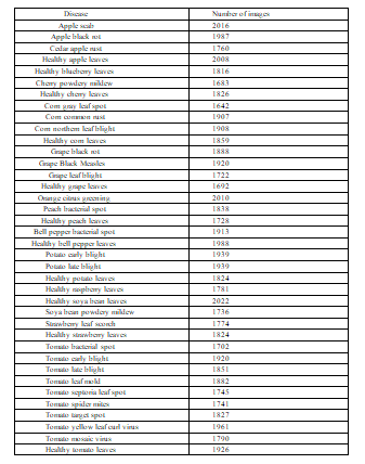
For this project, we will use the PlantVillage dataset available on Kaggle.

The PlantVillage dataset, a leaf disease image dataset, has been taken from Kaggle. The dataset consists of test an spot, black mold, grey mold, late blight, powdery mildew, and healthy leaves in apples, potato, tomato, corn, cherry, and soy crops. There are 70295 images in total, each with 227 * 227 pixels.

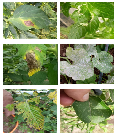
Several images of the leaf diseases are available in the dataset that has been used.

A few sample images from the dataset are shown below:

Getting Started with AlexNet

A CNN architecture named AlexNet was chosen as the 2012 LSVRC competition winner. Research teams compete to attain higher accuracy on various visual recognition tasks in the Large Scale Visual Recognition Challenge by evaluating their algorithms on a sizable dataset of annotated images (ImageNet). There are over 1.2 million training images, 50,000 validation images, and 150,000 testing images. By removing the central 256×256 patch from each image, the model builders imposed a fixed size of 256×256 pixels.
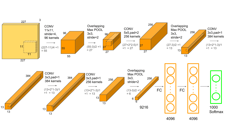
AlexNet’s architecture consists of 8 convolutional layers, of which 5 convolutional layers and three ANN layers. Each of the convolution layers is followed by a max pooling layer. Its architecture is easy to understand. It uses ReLu activation and involves overlapping max pooling. The following image shows the architecture of AlexNet.

Features of AlexNet:

• Kernels in the 2nd, 4th, and 5th convolution layers are interlinked to those kernels in the previous layers that lie on the same GPU.
• The neurons present in the fully connected layers are interconnected with each other.
• ReLu activation is applied to the output of every convolution layer and in the simple artificial neural network structure.

Usually, the sigmoid or tanh function is used as an activation function in deep learning networks. However, AlexNet employs a non-linear activation function called Rectified Linear Unit activation. The former activation functions saturate quickly, and training on GPUs using these functions is not easy, so non-linearity in ReLu helps with effective learning. The following equation gives the working functionality in ReLu:

𝑓(𝑥) = 𝑚𝑎𝑥(0, 𝑥)

The derivative of the above equation is 1 if x > 0 and 0 in other cases. Unlike sigmoid and tanh, which have the specific boundary of derivative values, the ReLu function has only two values for its derivative.
The vanishing gradient descent problem present when using sigmoid and tanh functions is not experienced during ReLu activation.

Local Response Normalization in AlexNet

Normalization is a crucial part of neural networks that use nonlinear activation functions. Nonlinear activation functions do not have a bounded set of outputs like linear ones, so we use normalization to restrict the unbounded activation outputs. Local response normalization helps the generalization process. ReLU was chosen as the activation function instead of the then-common tanh and sigmoid, which led to the usage of “local response normalization” (LRN) in the AlexNet architecture.
In addition to the aforementioned justification, the use of LRN was made to promote lateral inhibition. A neuron’s ability to lessen its neighbors’ action is a notion in neuroscience. This lateral inhibition function in DNNs is employed to perform local contrast enhancement such that the highest pixel values are used as local stimulation for the following layers. The pixel values of a feature map of a nearby neighborhood are square-normalized using LRN, a non-trainable layer.

Issues with AlexNet

Since the original architecture of AlexNet was developed using large amounts of data, overfitting is a problem when using this CNN. Data augmentation and dropout techniques were used to overcome this problem. By using dropout layers, the performance of the CNN architecture was seen to improve. The dropped attributes do not participate in forward and backward propagation, which reduces the complex co-adaptations of neurons. This allows the network to learn more robust features.

Using deep learning models like AlexNet can help in classifying plant diseases accurately.

The steps involved in this project include importing libraries, defining batch specifications, loading the dataset, building the AlexNet architecture, compiling the model, training and validation, saving the model, and testing it with a test image.

The AlexNet model consists of 5 convolutional layers, 3 max-pooling layers, and 2 dropout layers.

The model achieved a validation accuracy of 87% after 10 epochs.

The model can be saved for deployment and tested on new images for classification.

Overall, this project demonstrates how deep learning can be applied to solve real-world problems like plant disease classification.

Hence, it is crucial to detect them early so that necessary precautions can be taken.

Utilizing an automated system to classify images based on the disease is a modern approach to diagnosing plant diseases.

AlexNet demonstrates a high level of accuracy in categorizing images.

I trust you found my article on “Plant Disease Classification Using AlexNet” informative. Feel free to connect with me on LinkedIn here.

The media displayed in this article is not owned by Analytics Vidhya and is used with the author’s permission.

See also  GoSmart Brings AI to Fish Farmers Worldwide